


Blogs
Machine Learning in Credit Risk – Part 1: Cure Rate modelling
Date
April 9, 2021
Integrating Machine Learning methods into your credit risk modelling landscape is a great idea. It allows the user to find new, potentially non-linear, patterns in the data. However, simply applying Machine Learning methods onto a data set is not a guaranteed success. Most methods give fairly good results from the get-go. However, to get the most out of the data, the modeler should have a good understanding of these techniques. In this article we show that methods such as the Random Forest and Gradient Boosting outperform Logistic Regression in predicting the cure rate in LGD models. Besides that, we illustrate that Neural Networks are really data hungry!
Traditionally, credit risk models are based on regression methods that have been around for many years. In recent years, Machine Learning (ML) techniques popped up and showed great performance within fields such as fraud detection and healthcare. Potentially, ML methods could also improve the performance of credit risk models, thereby having a positive impact on the financial services industry. To investigate this, we developed a use case together with the Retail Bank Portfolio Management team of NIBC (using a simulated dataset based on characteristics of the NIBC retail mortgages portfolio). This is the first part of a two-part series blog, where we test several ML methods on a dataset in the context of Loss Given Default Modelling and evaluate the potential of ML techniques within credit risk modeling.
In this first article, we focus on the “cure rate” model, which is a model that aims to predict which of its lenders that are in default will (y = 1) or will not (y = 0) cure. Traditionally, a Logistic Regression is used to calculate the cure rate for each loan. By replacing this method with a ML model, we aim to improve the accuracy of the estimations, whilst still adhering to the framework set by the EBA.
Table of contents
4 Different Types of Machine Learning Models
For this research, we look at four different ML techniques to replace the traditional logistic regression: Decision Trees (DT), Random Forest (RF), Gradient Boosting using Decision Trees (XGBOOST), and Neural Networks (NN). The benchmark is the Logistic Regression (LR) model, which is currently commonly used within banks. Let’s take a quick look at all the techniques.
Decision Trees
DTs optimize many binary choices. At each node all remaining observations are allocated to two sub-nodes: values below a certain threshold follow one branch, and values above the threshold follow the other branch. It is key to optimize the criteria for each split, that is, which risk driver is used to split the data and what value is used as the decision boundary. The method has great interpretability since the tree shows all binary decisions. The key challenge in modelling DTs is to optimize the number of splits: how large will you allow the tree to be to maximize predictive power, while preventing overfitting.
Random Forest
The RF method is an ensemble method (i.e., a method that combines other ML methods) that uses many decision trees and combines their predictive power to improve the overall performance. How does this work? The RF method constructs all the trees using random subsets of the risk drivers to train the model. As a result, we obtain many different trees. It is not uncommon to use more than 1,000 trees! When a new data point (e.g., a defaulted mortgage) is evaluated, all the trained decision trees predict whether this mortgage will or will not cure. The combination (e.g., average or majority vote) of all these predictions becomes the final prediction of the RF. This method is a bit less intuitive than the DT technique since you no longer rely on a single tree. However, once you grasp that concept, the RF method becomes a powerful method, since the method generally performs better than using a single tree DT.
Gradient Boosting
Gradient boosting, like random forest, is an ensemble method that combines many decision trees in its calculation. The difference between gradient boosting and random forest lies in the way that the decision trees are constructed. Random forest creates its decision trees independently from each other using various sub-samples. In contrast, the decision trees in gradient boosting are created iteratively. The gradient boosting algorithm starts with a single decision tree. A second tree is then built that aims to minimize any errors that were made by the first decision tree. The thought is that combining these two trees leads to a better model than a single decision tree. This step is then repeated numerous times in order to minimize any errors made by each subsequent model. In this blog XGBoost, a well-known gradient boosting technique, is used.
Neural Networks
NNs sound complicated and impossible to grasp. However, they are just networks of linear regressions! The model connects the input data to the first layer and assigns weights to each observation. At each layer multiple regressions, which are represented as ‘neurons’, are stacked and the regressions results are weighted, combined and serve as input for the next layer. At the final node, the results are combined and transformed to obtain the desired result, e.g., classification or regression. Since the structure of NNs consists of multiple layers and neurons, the method uses many parameters. As a result, NNs need sufficient data to excel and besides that you need to be careful to prevent overfitting, but we will skip that topic for now.
The weights are key: each iteration of the model, the weights are updated to improve model performance. For example, the weight of a risk driver on the regression in one of the nodes in the first layer might decrease after an iteration to increase overall model performance. However, the model does not explain why this allocation of weights works best. Therefore, it is difficult to get a feeling for what goes into each layer and what comes out of each layer. Hence, the method earns the reputation of being a “black box”. You can now understand why neural networks can decipher complex relations: they are great at discovering non-linear relationships. A visual representation is given in Figure 1.

Does Machine Learning Improve the Prediction Performance?
To assess whether ML methods can improve the prediction performance, we calculated the out-of-sample AUC metric for each different prediction method and compare these methods with the traditional Logistic Regression. In Figure 2, we show the AUC for each model for different sized datasets. One thing immediately stands out: Logistic Regression is hard to beat! The RF and XGBoost methods perform better only if there is a substantial number of observations. Why is that? Aren’t ML methods always the better choice?
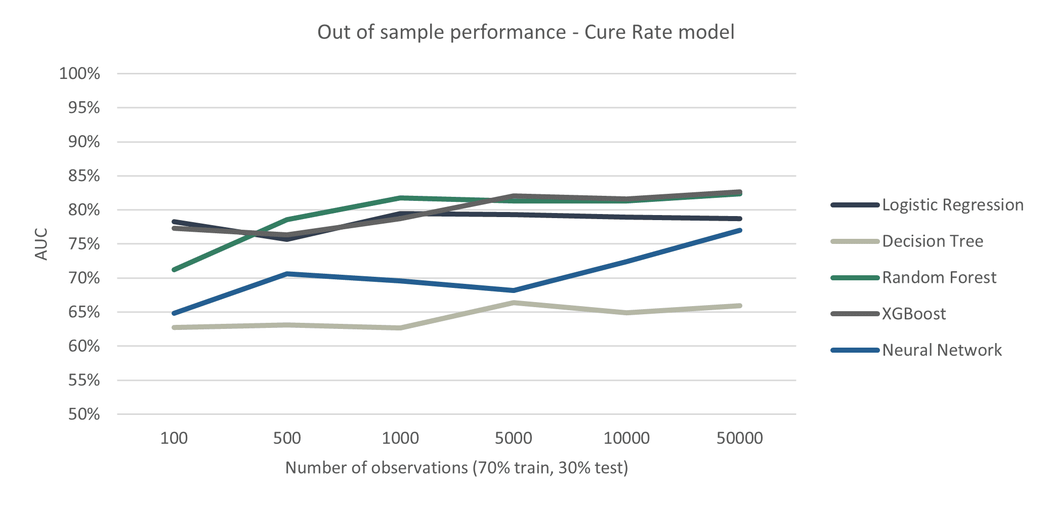
Generally, the AUC score improves with an increase in the number of observations, which is obvious, since more observations give us more information about relevant drivers for the cure rate. In particular, the pace at which the models learn from data shows an interesting pattern: the traditional Logistic Regression performs quite well with small datasets and improves only marginally once the number of observations grows, while the ML methods seem to grow steadily once the number of observations grows, which enables the RF and XGBoost methods to achieve a higher performance than the traditional Logistic Regression. This is most likely due to the nature of ML methods being more complex, requiring more data whilst allowing the model to capture more non-linear and complex patterns once there is enough data.
One of the other ML methods, the Neural Network, however, seems to require a lot of data. The performance increases substantially when the number of observations grows, and at 50,000 observations it seems to be almost on par with the Logistic Regression. Possibly, when we would have had even more observations, the NN could be the best-performing method.
Another interesting finding is that the DT method performs bad, which is to be expected as a DT is a simplistic model, too simplistic for predicting the cure rate. It is remarkable is that the best-performing models, RF and XGBoost, consist of many of these bad-performing DT’s. So, in this case, a lot of bad predictors combined make a good prediction model! That is the magic of ensemble methods…
Long story short: ML methods require more data but can also learn more complex patterns resulting in a better-performing model compared to the traditional Logistic Regression, if there is enough data. Banks generally have access to a lot of data so they could benefit greatly from ML methods.
A perk of the Logistic Regression method, however, is its interpretability: the influence of each risk driver on the overall result is easily derived as the relationship between the risk drivers and the cure rate is log-linear. For ML methods, this is more complex as each risk driver affects the cure rate through many different patterns. This is the reason that ML methods have a reputation of being a “black box”. However, most methods allow for some interpretability. We examine the RF model here as a use-case. While the RF cannot show the direct relationship between risk drivers and the cure rate, we can infer the magnitude of impact of each risk driver. Figure 3 shows that risk drivers NHG, Arrears, Number of Months in Arrears (ArrearsPast12Months), and Seasoning mostly influence the prediction that comes from the RF method.

How can Machine Learning Contribute to Credit Risk modelling?
Should you include ML models into your modelling landscape? Obviously, the answer is yes. Two main reasons are as follows:
- Governing bodies keep a keen eye on the developments of ML methods since they acknowledge the potential of the methods to increase stability of the financial industry. Regulations might shift to allow for more use of these methods, or development of ML methods reaches sufficient levels that they fit into the current regulatory framework. Development cycles for large organizations takes years, hence an organization should act now to gain a competitive advantage over its competitors!
- An ML model could be used to challenge the existing, traditional, method, e.g., during the model validation phase. As ML methods can find patterns within data between variables in ways that traditional methods are unable to, ML models can show the potential that lies within the available data. This could be a starting point to dive deeper into the current data and variables that are defined to improve the traditional method.
What’s Next?
In this blogpost we showed how ML can be used to improve a traditional cure rate model. We replaced a Logistic Regression by an ML method within the LGD framework, adhering to the EBA guidelines. What happens if we let the ML method predict the LGD directly? Without the use of the LGD formula and using more unconventional yet innovative methods! While this is not allowed because of regulatory restrictions, it could form an interesting starting point for discovering future possibilities within the field of credit risk modelling. We dive into these opportunities in the next part of this blog posts series.
Are you interested in how ML techniques would perform on your data? We are happy to help you get the most out of your data using innovative techniques! Please get in contact with us using the contact details below.
Resources
The AUC metric measures the capacity of a model to distinguish “cured” loans from “non-cured” loans (on a scale of 0.5 to 1.0).
Date
April 9, 2021
Integrating Machine Learning methods into your credit risk modelling landscape is a great idea. It allows the user to find new, potentially non-linear, patterns in the data. However, simply applying Machine Learning methods onto a data set is not a guaranteed success. Most methods give fairly good results from the get-go. However, to get the most out of the data, the modeler should have a good understanding of these techniques. In this article we show that methods such as the Random Forest and Gradient Boosting outperform Logistic Regression in predicting the cure rate in LGD models. Besides that, we illustrate that Neural Networks are really data hungry!
Traditionally, credit risk models are based on regression methods that have been around for many years. In recent years, Machine Learning (ML) techniques popped up and showed great performance within fields such as fraud detection and healthcare. Potentially, ML methods could also improve the performance of credit risk models, thereby having a positive impact on the financial services industry. To investigate this, we developed a use case together with the Retail Bank Portfolio Management team of NIBC (using a simulated dataset based on characteristics of the NIBC retail mortgages portfolio). This is the first part of a two-part series blog, where we test several ML methods on a dataset in the context of Loss Given Default Modelling and evaluate the potential of ML techniques within credit risk modeling.
In this first article, we focus on the “cure rate” model, which is a model that aims to predict which of its lenders that are in default will (y = 1) or will not (y = 0) cure. Traditionally, a Logistic Regression is used to calculate the cure rate for each loan. By replacing this method with a ML model, we aim to improve the accuracy of the estimations, whilst still adhering to the framework set by the EBA.
Table of contents
4 Different Types of Machine Learning Models
For this research, we look at four different ML techniques to replace the traditional logistic regression: Decision Trees (DT), Random Forest (RF), Gradient Boosting using Decision Trees (XGBOOST), and Neural Networks (NN). The benchmark is the Logistic Regression (LR) model, which is currently commonly used within banks. Let’s take a quick look at all the techniques.
Decision Trees
DTs optimize many binary choices. At each node all remaining observations are allocated to two sub-nodes: values below a certain threshold follow one branch, and values above the threshold follow the other branch. It is key to optimize the criteria for each split, that is, which risk driver is used to split the data and what value is used as the decision boundary. The method has great interpretability since the tree shows all binary decisions. The key challenge in modelling DTs is to optimize the number of splits: how large will you allow the tree to be to maximize predictive power, while preventing overfitting.
Random Forest
The RF method is an ensemble method (i.e., a method that combines other ML methods) that uses many decision trees and combines their predictive power to improve the overall performance. How does this work? The RF method constructs all the trees using random subsets of the risk drivers to train the model. As a result, we obtain many different trees. It is not uncommon to use more than 1,000 trees! When a new data point (e.g., a defaulted mortgage) is evaluated, all the trained decision trees predict whether this mortgage will or will not cure. The combination (e.g., average or majority vote) of all these predictions becomes the final prediction of the RF. This method is a bit less intuitive than the DT technique since you no longer rely on a single tree. However, once you grasp that concept, the RF method becomes a powerful method, since the method generally performs better than using a single tree DT.
Gradient Boosting
Gradient boosting, like random forest, is an ensemble method that combines many decision trees in its calculation. The difference between gradient boosting and random forest lies in the way that the decision trees are constructed. Random forest creates its decision trees independently from each other using various sub-samples. In contrast, the decision trees in gradient boosting are created iteratively. The gradient boosting algorithm starts with a single decision tree. A second tree is then built that aims to minimize any errors that were made by the first decision tree. The thought is that combining these two trees leads to a better model than a single decision tree. This step is then repeated numerous times in order to minimize any errors made by each subsequent model. In this blog XGBoost, a well-known gradient boosting technique, is used.
Neural Networks
NNs sound complicated and impossible to grasp. However, they are just networks of linear regressions! The model connects the input data to the first layer and assigns weights to each observation. At each layer multiple regressions, which are represented as ‘neurons’, are stacked and the regressions results are weighted, combined and serve as input for the next layer. At the final node, the results are combined and transformed to obtain the desired result, e.g., classification or regression. Since the structure of NNs consists of multiple layers and neurons, the method uses many parameters. As a result, NNs need sufficient data to excel and besides that you need to be careful to prevent overfitting, but we will skip that topic for now.
The weights are key: each iteration of the model, the weights are updated to improve model performance. For example, the weight of a risk driver on the regression in one of the nodes in the first layer might decrease after an iteration to increase overall model performance. However, the model does not explain why this allocation of weights works best. Therefore, it is difficult to get a feeling for what goes into each layer and what comes out of each layer. Hence, the method earns the reputation of being a “black box”. You can now understand why neural networks can decipher complex relations: they are great at discovering non-linear relationships. A visual representation is given in Figure 1.
Does Machine Learning Improve the Prediction Performance?
To assess whether ML methods can improve the prediction performance, we calculated the out-of-sample AUC metric for each different prediction method and compare these methods with the traditional Logistic Regression. In Figure 2, we show the AUC for each model for different sized datasets. One thing immediately stands out: Logistic Regression is hard to beat! The RF and XGBoost methods perform better only if there is a substantial number of observations. Why is that? Aren’t ML methods always the better choice?
Generally, the AUC score improves with an increase in the number of observations, which is obvious, since more observations give us more information about relevant drivers for the cure rate. In particular, the pace at which the models learn from data shows an interesting pattern: the traditional Logistic Regression performs quite well with small datasets and improves only marginally once the number of observations grows, while the ML methods seem to grow steadily once the number of observations grows, which enables the RF and XGBoost methods to achieve a higher performance than the traditional Logistic Regression. This is most likely due to the nature of ML methods being more complex, requiring more data whilst allowing the model to capture more non-linear and complex patterns once there is enough data.
One of the other ML methods, the Neural Network, however, seems to require a lot of data. The performance increases substantially when the number of observations grows, and at 50,000 observations it seems to be almost on par with the Logistic Regression. Possibly, when we would have had even more observations, the NN could be the best-performing method.
Another interesting finding is that the DT method performs bad, which is to be expected as a DT is a simplistic model, too simplistic for predicting the cure rate. It is remarkable is that the best-performing models, RF and XGBoost, consist of many of these bad-performing DT’s. So, in this case, a lot of bad predictors combined make a good prediction model! That is the magic of ensemble methods…
Long story short: ML methods require more data but can also learn more complex patterns resulting in a better-performing model compared to the traditional Logistic Regression, if there is enough data. Banks generally have access to a lot of data so they could benefit greatly from ML methods.
A perk of the Logistic Regression method, however, is its interpretability: the influence of each risk driver on the overall result is easily derived as the relationship between the risk drivers and the cure rate is log-linear. For ML methods, this is more complex as each risk driver affects the cure rate through many different patterns. This is the reason that ML methods have a reputation of being a “black box”. However, most methods allow for some interpretability. We examine the RF model here as a use-case. While the RF cannot show the direct relationship between risk drivers and the cure rate, we can infer the magnitude of impact of each risk driver. Figure 3 shows that risk drivers NHG, Arrears, Number of Months in Arrears (ArrearsPast12Months), and Seasoning mostly influence the prediction that comes from the RF method.
How can Machine Learning Contribute to Credit Risk modelling?
Should you include ML models into your modelling landscape? Obviously, the answer is yes. Two main reasons are as follows:
- Governing bodies keep a keen eye on the developments of ML methods since they acknowledge the potential of the methods to increase stability of the financial industry. Regulations might shift to allow for more use of these methods, or development of ML methods reaches sufficient levels that they fit into the current regulatory framework. Development cycles for large organizations takes years, hence an organization should act now to gain a competitive advantage over its competitors!
- An ML model could be used to challenge the existing, traditional, method, e.g., during the model validation phase. As ML methods can find patterns within data between variables in ways that traditional methods are unable to, ML models can show the potential that lies within the available data. This could be a starting point to dive deeper into the current data and variables that are defined to improve the traditional method.
What’s Next?
In this blogpost we showed how ML can be used to improve a traditional cure rate model. We replaced a Logistic Regression by an ML method within the LGD framework, adhering to the EBA guidelines. What happens if we let the ML method predict the LGD directly? Without the use of the LGD formula and using more unconventional yet innovative methods! While this is not allowed because of regulatory restrictions, it could form an interesting starting point for discovering future possibilities within the field of credit risk modelling. We dive into these opportunities in the next part of this blog posts series.
Are you interested in how ML techniques would perform on your data? We are happy to help you get the most out of your data using innovative techniques! Please get in contact with us using the contact details below.
Resources
The AUC metric measures the capacity of a model to distinguish “cured” loans from “non-cured” loans (on a scale of 0.5 to 1.0).
Talk to our experts
Let's create real impact together with data and AI

Financial Services Lead
Henriette Claus
Talk to our experts
Let's create real impact together with data and AI
Financial Services Lead
Henriette Claus